Physical Simulation in ChronosDB
Physical Environment
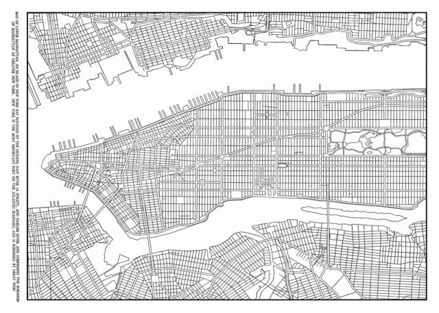
We use a traditional example of a road grid: an artificial road map resembling the Manhattan Grid, New York City, similar to [30].
We represent a road grid by a 2-d array called "tca.lane". It stores cells with the following values (indicators):
- -1 or NoData (white) — impassible area
- 0 (green)— a cell that belongs to a road with west-east moving direction
- 1 (purple)— a cell that belongs to a road with south-north moving direction
- 2 (cyan)— a road intersection
- 3 (red)— traffic lights
We take a traditional cell size of 7.5 meters [15].
We assume impassible parts to be 15 x 15 cells in size.
Each road has 3 lanes (a lane width is 1 cell).
Manhattan Island is 22.7 square miles (59 sq km) in area, 13.4 miles (21.6 km) long and 2.3 miles (3.7 km) wide at its widest (near 14th Street) link.
We take the shape of the "tca.lane" array to be 256 x 4096 cells.
It is a realistic shape yielding an area of about 1.9 km x 30.7 km.
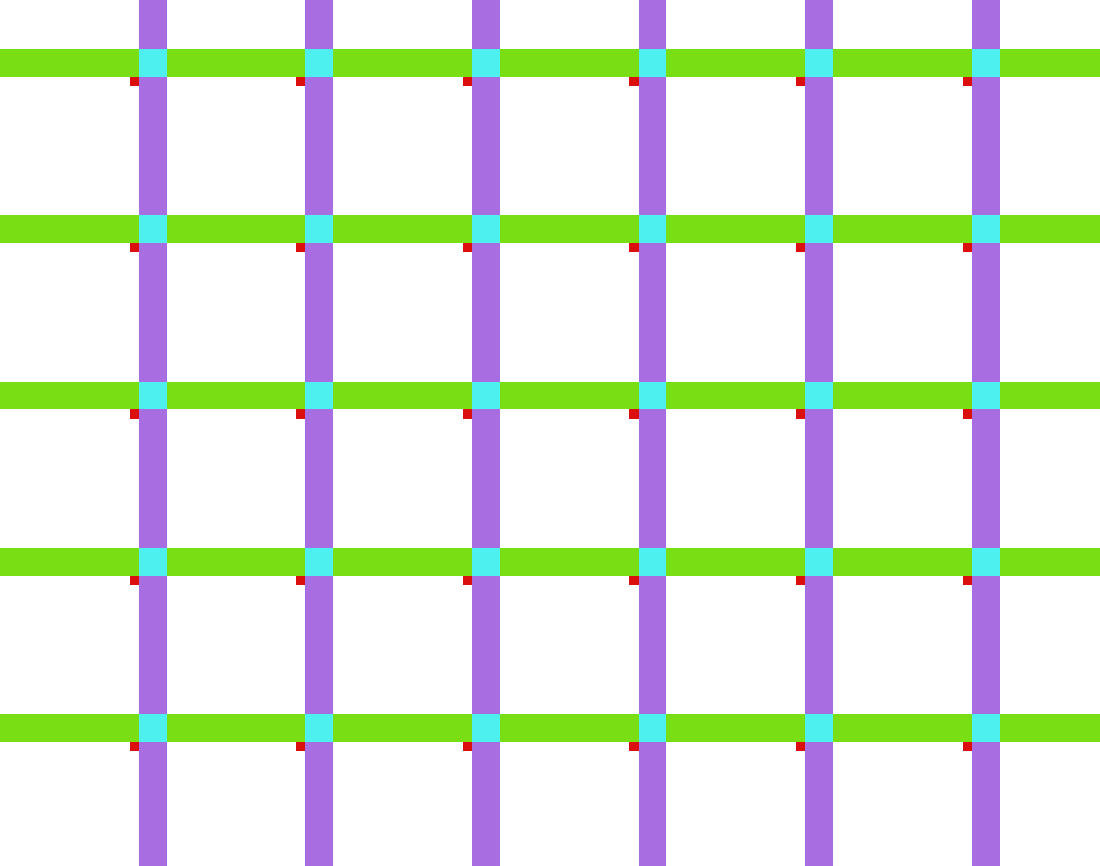
A portion of the "tca.lane" array in ChronosDB
(The Cellular Automaton Lattice)
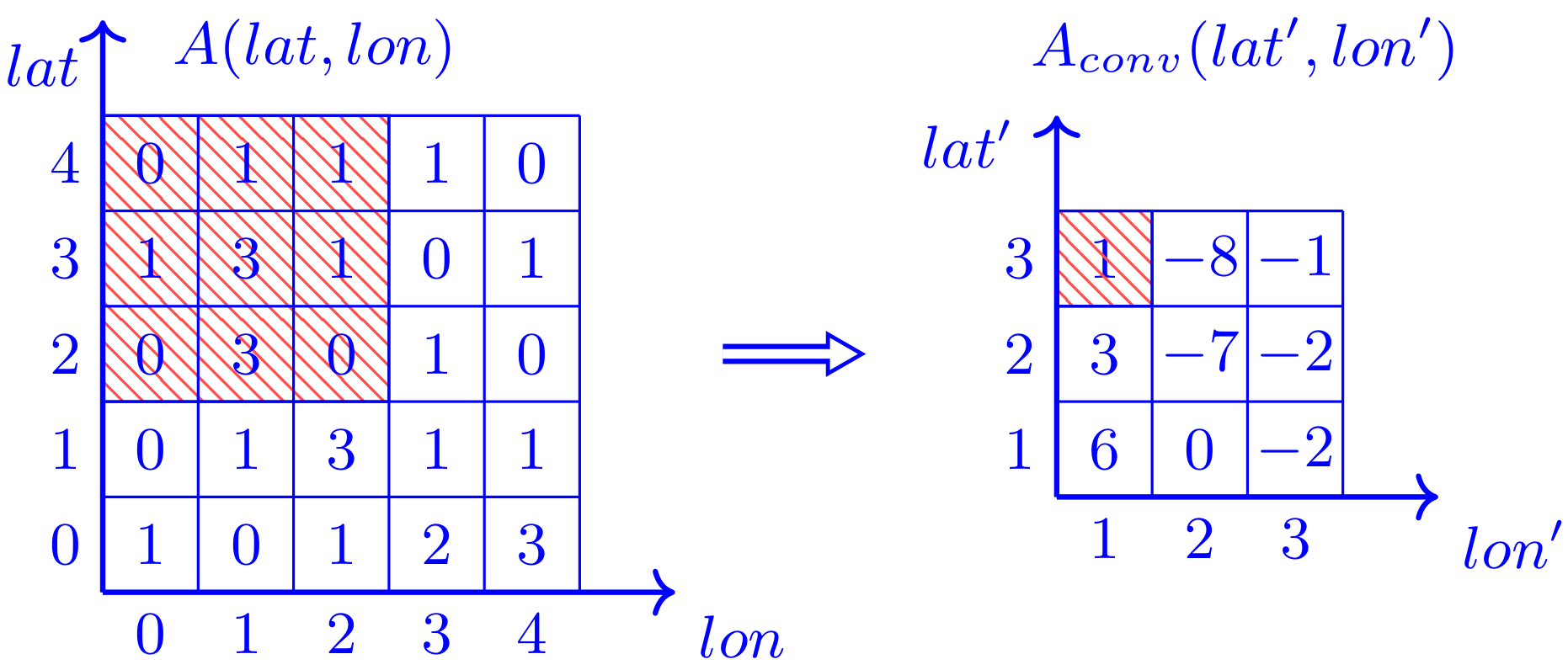
It is possible to generate such a 2-d array by running the convolution operator with the following UDF:
int BW = 15;
int NLANES = 3;

int localX = windows.input(0).getArrayX() % (BW + NLANES);
int localY = windows.input(0).getArrayY() % (BW + NLANES);

Double result = null;

if (localX == BW - 1 && localY == 0) {
    result = 3d;
} else if (localX < BW && localY < BW) {
    result = null;
} else if (localX >= BW && localY >= BW) {
    result = 2d;
} else if (localX >= BW) {
    result = 1d;
} else if (localY >= BW) {
    result = 0d;
}

windows.output(0).set(result, 0, 0);
Initialization
We create initial conditions by distributing vehicles over the grid cells using our convolution operator.
First, for each cell, we decide whether it should contain a vehicle's rear bumper with probability > 0.85.
We omit cells that belong to road intersections at this initial step.
Next, we should assign a length to the newly created vehicle.
The length of a vehicle cannot be larger than its distance to the closest obstacle along the moving direction:
the next vehicle on the same lane, grid border, or a road intersection.
However, we cannot assign lengths to vehicles during this stage: cells are processed in parallel,
so vehicles appear on the grid independently of each other.
There is no warranty that a vehicle will appear in front of the newly created vehicle after
we check the above condition.
Hence, we setup initial conditions in 2 stages.
At the first stage, we randomly decide whether a cell should contain a vehicle's rear bumper.
At the second stage, when all vehicles' positions are already known and fixed,
we assign lengths to vehicles by checking the required inter-obstacle distance constraint.
The following array DBMS query, consisting of 3 convolution operators (calc),
will create two 2-d arrays tca.length and tca.speed
that will contain vehicles' lengths and speeds.
This query generates the initial conditions for the simulation.
calc tca.lane $pos -classfile "TCA.java" -method_name putVehicle -ot Int16
calc $pos tca.length -classfile "TCA.java" -method_name setLength -xWindowSize 3 -yWindowSize 3 -ot Int16
calc $pos tca.speed -classfile "TCA.java" -method_name setSpeed -ot Int16
The window size (3 x 3) is specified only for the operator that generates vehicles' lengths as it has to check its neighborhood.
$pos is a temporary 2-d array that contains vehicles' positions at which the following operators will generate the vehicles' speeds and lengths.
Note that "tca.speed" and "tca.length" arrays are being generated in parallel using the "$pos" array as an input.
At the first stage, we apply the following rules on each cell of the "tca.lane" array and produce the following values
which we store in the intermediate "$pos" array:
- NoData ⇒ skip (happens automatically)
- 2 (road intersection) ⇒ 2
- 1 & vehicle's rear bumper is decided to be in this cell ⇒ 1
- 1 & no vehicle at this cell ⇒ -1
- 0 & vehicle's rear bumper is decided to be in this cell ⇒ 0
- 0 & no vehicle at this cell ⇒ -2
After the first stage, the resulting array "$pos" contains not only the vehicles' positions,
but also information about the moving direction & road intersections (road layout).
In this way, we reduce the cost of the next stage by avoiding the join operator with the
"tca.lane" and "$pos" arrays in order to obtain both road layout and vehicle positions.
The procedure of assigning a length to a south-north moving vehicle is exactly the same if we rotate the window by 270°
counter-clockwise (y-axis goes from top to bottom).
Therefore, we first determine the vehicle's moving direction, rotate the window if necessary,
and then apply the same logic to compute the vehicle length.
To complete the initialization, we need to set initial speeds to vehicles.
A vehicle speed can take any allowed value (0..3) at this stage,
as it will be immediately corrected by applying move forward rules once the simulation starts.
Java UDFs are in the TCA.java file
    public void putVehicle(ConvolveWindows w) {
        double laned = w.input(0).get(0, 0);
        int lane = (int) laned;
        boolean is = w.input(0).random().nextDouble() > 0.85;

        double result = Double.MAX_VALUE;
        if (lane == LANE_TRAFFIC_LIGHTS) result = 4.;
        if (lane == LANE_ROAD_CROSSING) result = 2.;
        if (lane == LANE_SOUTH_NORTH && is) result = 1.;
        if (lane == LANE_SOUTH_NORTH && !is) result = -1.;
        if (lane == LANE_WEST_EAST && is) result = 0.;
        if (lane == LANE_WEST_EAST && !is) result = -2.;

        w.output(0).set(result, 0, 0);
    }

    public void setLength(ConvolveWindows w) {
        InputConvolveWindow win = w.input(0);
        double val = win.get(0, 0);
        if (val != 1 && val != 0) {
            if (val == 4) {
                // traffic lights
                w.output(0).set((double) 0, 0, 0);
            } else {
                w.output(0).set(null, 0, 0);
            }
            return; // no vehicle
        }
        // a south-north moving vehicle, just rotate the window
        if (val == 1) win = win.rotate(ConvolveWindow.Degrees._270);
        int cellsToClosestVehicle = 1;
        for (int i = 1; i < MAX_VEHICLE_LENGTH; i++) {
            Double next = win.get(i, 0);
            if (next == null || next >= 0) break;
            cellsToClosestVehicle++;
        }
        int vehicleLength = win.random().nextInt(cellsToClosestVehicle) + 1;
        w.output(0).set((double) (vehicleLength), 0, 0);
    }

    public void setSpeed(ConvolveWindows w) {
        double val = w.input(0).get(0, 0);
        Double output = null;
        if (val == 1 || val == 0) {
            output = (double) w.input(0).random().nextInt(4);
        } else {
            if (val == 4) {
                // traffic lights
                output = (double) (200 + w.output(0).random().nextInt(2) + 1);
            }
        }
        w.output(0).set(output, 0, 0);
    }
The fragment of the generated tca.length array is presented below.
Only cells that are occupied by vehicles' rear bumpers are shown.
Length cells are colored as follows:
- 1 (green)— a vehicle is 1 cell long
- 2 (blue)— a vehicle is 2 cells long
- 3 (red)— a vehicle is 3 cells long
For example, if you see a red cell on a west-east moving lane,
this cell and two cells to the right are occupied by a vehicle.
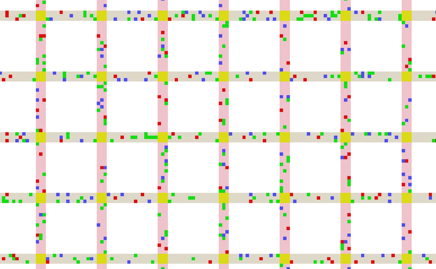
A fragment of the initial "tca.length" array
("tca.lane" array is used as a background, e.g. yellow indicates a road intersection, etc.)
Below is the same fragment of the lattice, but with initial speeds of vehicles.
Speed cells are colored as follows
- 0 (green)— vehicle's speed is 0
- 1 (purple)— vehicle's speed is 1
- 2 (cyan)— vehicle's speed is 2
- 3 (red)— vehicle's speed is 3
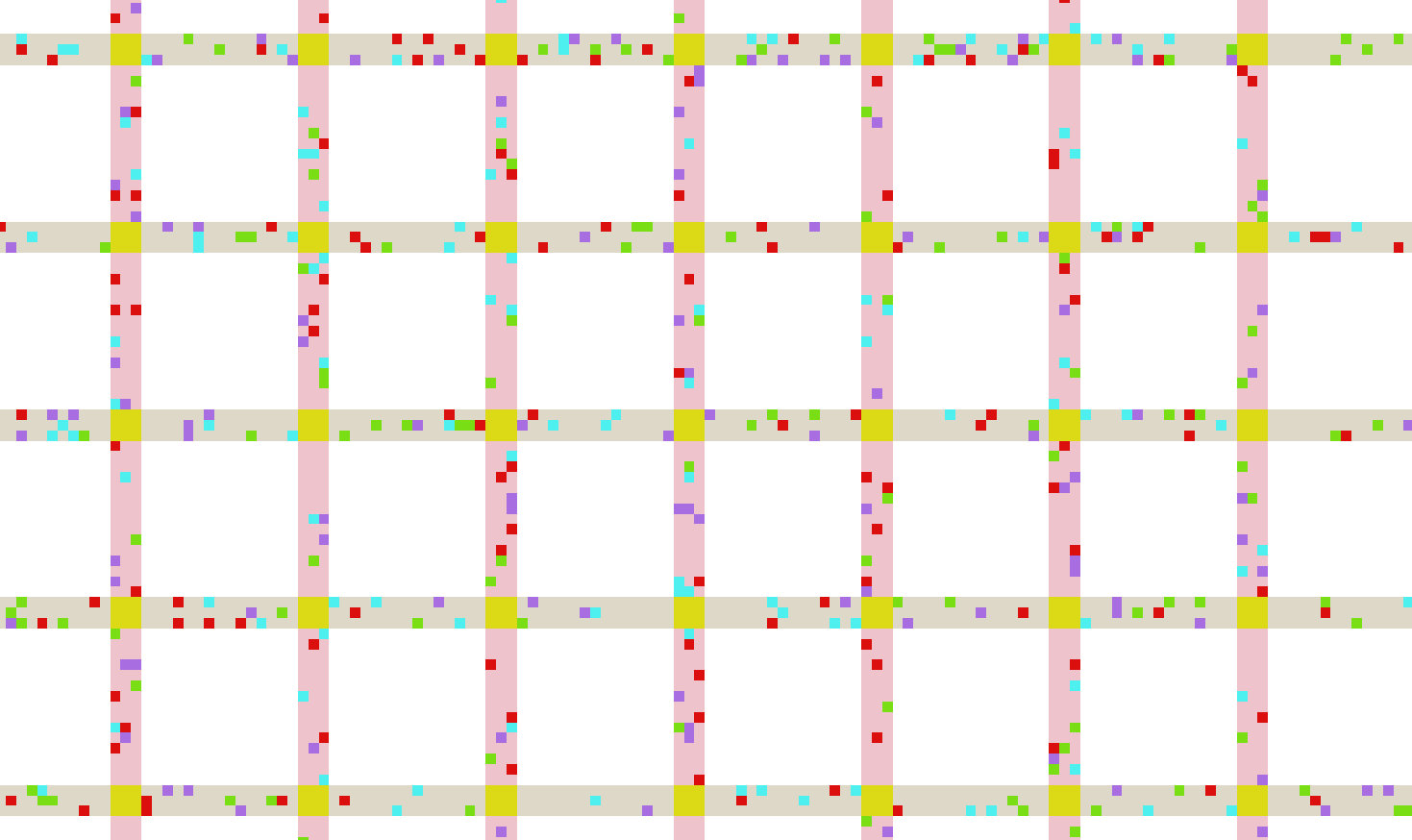
A fragment of the initial "tca.speed" array
("tca.lane" array is used as a background, e.g. yellow indicates a road intersection, etc.)
We created array visualizations in
 by directly accessing arrays that are under the control of ChronosDB.
This demonstrates the interoperability of ChronosDB with other software
from which physical simulations, running inside ChronosDB, readily benefit.
by directly accessing arrays that are under the control of ChronosDB.
This demonstrates the interoperability of ChronosDB with other software
from which physical simulations, running inside ChronosDB, readily benefit.
Advancing Simulation by ChronosDB
The simulation consists of the following steps repeated in each cycle N times:
- Each vehicle is advanced several steps forward
- Each vehicle decides whether to turn left and possibly turns left
- Each vehicle decides whether to turn right and possibly turns right
- Traffic lights change their color
- Advance the timer
The following is the UDF in the native array DBMS language
cp tca.speed $speed
cp tca.length $length

val {window} "-xWindowSize 11 -yWindowSize  11"

foreach {step} -from 0 -to 100
begin
    calc tca.lane:in $speed:in $length:in tca.temperature:in \
            --overwrite $speed_move:out $length_move:out     \
            -ot Int16 {window} -classfile "TCA.java"                     \
            -method_name moveForwardPhase
    calc tca.lane:in $speed_move:in $length_move:in  \
            --overwrite $speed_left:out $length_left:out     \
            -ot Int16 {window} -classfile "TCA.java"             \
            -method_name turnLeftPhase
    calc tca.lane:in $speed_left:in $length_left:in                  \
            --overwrite $speed_lights:out $length_lights:out      \
            -ot Int16 {window} -classfile "TCA.java"                     \
            -method_name turnRightPhase
    calc tca.lane:in $speed_lights:in $length_lights:in \
            --overwrite $speed:out $length:out                 \
            -ot Int16 {window} -classfile"TCA.java"            \
            -method_name lightsPhase
    append $speed speedh
    append $length lenh
end
References
- [30] Ozan K Tonguz, Wantanee Viriyasitavat, and Fan Bai. 2009. Modeling urban traffic: a cellular automata approach. IEEE Communications Magazine 47, 5 (2009), 142–150.
- [15] Sven Maerivoet and Bart De Moor. 2005. Cellular automata models of road traffic. Physics reports 419, 1 (2005), 1–64.